City of toronto maintains a variety of interesting datasets on open.toronto.ca/datasets . In this article I explore the Active Permits and Cleared Permits datasets which contain records of all building permit applications of Toronto since 2000.
let’s start by loading the active permits dataset and taking a look at the features. I recommend you take a look at the readme file as well.
permits = pd.read_csv("datasets/activepermits.csv")

Index(['PERMIT_NUM', 'REVISION_NUM', 'PERMIT_TYPE', 'STRUCTURE_TYPE', 'WORK',
       'STREET_NUM', 'STREET_NAME', 'STREET_TYPE', 'STREET_DIRECTION',
       'POSTAL', 'GEO_ID', 'WARD_GRID', 'APPLICATION_DATE', 'ISSUED_DATE',
       'COMPLETED_DATE', 'STATUS', 'DESCRIPTION', 'CURRENT_USE',
       'PROPOSED_USE', 'DWELLING_UNITS_CREATED', 'DWELLING_UNITS_LOST',
       'EST_CONST_COST', 'ASSEMBLY', 'INSTITUTIONAL', 'RESIDENTIAL',
       'BUSINESS_AND_PERSONAL_SERVICES', 'MERCANTILE', 'INDUSTRIAL',
       'INTERIOR_ALTERATIONS', 'DEMOLITION'],
      dtype='object')
Most frequent types of permits
permits["PERMIT_TYPE"].value_counts().iloc[:10].plot(kind="bar",rot=90)
Most frequent street names
permits["STREET_NAME"].value_counts().head(10)

YONGE       5433
SHEPPARD    3819
BLOOR       3310
DUNDAS      3092
KING        3074
QUEEN       2965
LAWRENCE    2352
BAY         2160
EGLINTON    2140
ST CLAIR    1884
Name: STREET_NAME, dtype: int64
Contributions of occupancy
the last columns in the table are the square meters of the area for each type of occupancy. for example one of the permits has 157.00 square meters of RESIDENTIAL occupancy.
here are the percentages for the whole table.
occupancy = permits.loc[:,"ASSEMBLY":].sum(axis=0)
occupancy = round((occupancy/ occupancy.sum()) *100,2)
occupancy.sort_values(ascending=False).astype(str) + "%"


RESIDENTIAL                       42.95%
INTERIOR_ALTERATIONS              18.01%
INDUSTRIAL                        15.39%
BUSINESS_AND_PERSONAL_SERVICES    12.17%
DEMOLITION                         5.48%
ASSEMBLY                           2.58%
MERCANTILE                         1.94%
INSTITUTIONAL                      1.47%
dtype: object
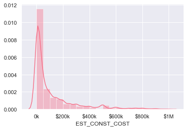
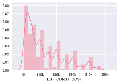
Distribution of construction cost
Here we scale the construction costs to $1/1000 and then limit it to under 2 million dollars. The mean turns out to be at $506k and there are some picks on rounded values like $10k, $20k, $30k.
cost = permits["EST_CONST_COST"].dropna()
cost = cost[ cost.str.isnumeric()].astype(float)
cost /= 1000 # scale it to thousands of dollars
cost = cost[(cost>0) & (cost<1000)]
# cost = cost[(cost>0.001) & (cost<50)] # under $50k
ax = sns.distplot(cost,bins=20)
# ax.set(xticklabels=["","0k","$10k","$20k","$30k","$40k","$50k"])
ax.set(xticklabels=["","0k","$200k","$400k","$600k","$800k","$1M"])
cost.describe()


count     89657.000000
mean        506.999859
std        6607.660147
min           0.000000
25%           1.000000
50%          15.000000
75%         120.000000
max      595875.683000
Name: EST_CONST_COST, dtype: float64
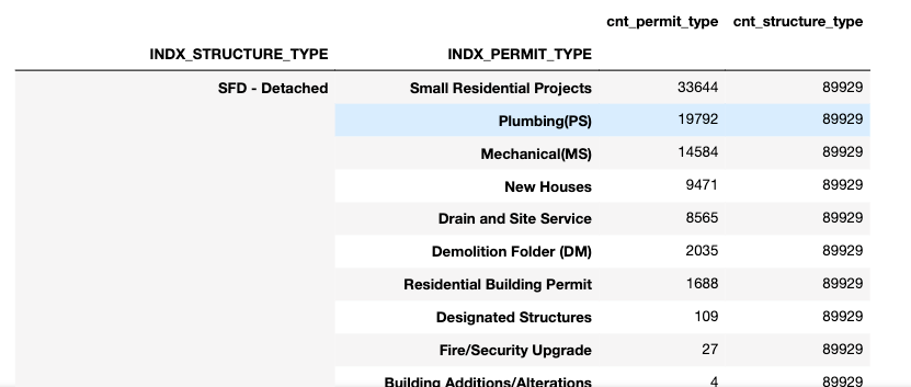
Most frequent structure types and permit types
pd.set_option('display.max_rows', 1000)
structure_permit_groups = permits.groupby(["STRUCTURE_TYPE","PERMIT_TYPE"])\
                                 .agg({ "PERMIT_TYPE":"count"})
structure_permit_groups.index.names=["INDX_STRUCTURE_TYPE","INDX_PERMIT_TYPE"]
structure_permit_groups["cnt_structure_type"] = structure_permit_groups.groupby(["INDX_STRUCTURE_TYPE"])\
                                                                       .transform(np.sum)
structure_permit_groups.columns = ["cnt_permit_type","cnt_structure_type"]
structure_permit_groups = structure_permit_groups.sort_values(["cnt_structure_type","cnt_permit_type"]
                                                              ,ascending=False)
Trend of permits over time
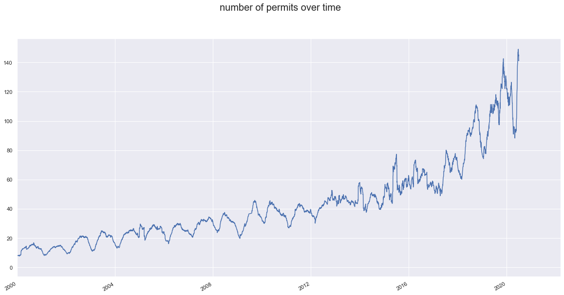
our main goal for this article is to gain some perspective on how the number and proportions of permits are changing over time. we start by looking into aggregate number of all permits together. The seasonal pattern is pretty interesting but doensn’t tell us anything about whats happening in each category .
permits["APPLICATION_DATE"] = pd.to_datetime(permits["APPLICATION_DATE"],format="%Y%m%d000000")
dates = permits["APPLICATION_DATE"].value_counts()
dates = dates.sort_index()
fig, ax  = plt.subplots(1)
fig.suptitle("number of permits over time",fontsize=20)
dates.rolling(50).mean().plot(figsize=(20,10),ax=ax)
ax.set_xlim(pd.Timestamp("2000-01-01"))
Categories of permits and their trend over time
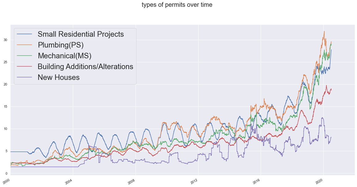
First we find the most active types of permits. and then we can go ahead and plot each of them and see how they’re changing together.
frequent_permit_types= permits["PERMIT_TYPE"].value_counts().iloc[:5].index.tolist()
frequent_permit_types

['Small Residential Projects',
 'Plumbing(PS)',
 'Mechanical(MS)',
 'Building Additions/Alterations',
 'New Houses']
fig, axes  = plt.subplots(1,figsize=(20,10))

fig.suptitle("types of permits over time",fontsize=20)
sns.set_palette("husl")

for i,permit_type in enumerate(frequent_permit_types):
    type_trend = permits[permits["PERMIT_TYPE"]==permit_type]["APPLICATION_DATE"].value_counts()
    type_trend.sort_index(inplace=True)
    ax = type_trend.rolling(100).mean().plot(label=permit_type)
    ax.set_xlim(pd.Timestamp("2000-01-01"))

plt.legend( prop={'size': 24})
The seasonal trend of Small Residential Projects is pretty strong. which totally makes sense in the case of outdoor projects. let’s take a look at the work column:
permits[permits["PERMIT_TYPE"]=="Small Residential Projects"]["WORK"].value_counts()

Multiple Projects                           18437
Interior Alterations                         7563
Addition(s)                                  6978
Garage                                       3504
Party Wall Admin Permits                     3299
Other(SR)                                    2702
Porch                                        2099
Deck                                         1916
Underpinning                                 1731
Unknown                                      1413
Accessory Building(s)                         820
Second Suite (New)                            715
Walk-Out Stair                                651
Fire Damage                                   532
Finishing Basements                           389
Carport                                       326
Canopy                                        281
New Laneway / Rear Yard Suite                 111
Pool Fence Enclosure                           98
Types of CURRENT_USE
the CURRENT_USE column gives us a good insight on what most of these permits are all about. let’s take a quick look at the most frequent ones.
permits["CURRENT_USE"].value_counts().head(20)

Sfd                       48593
Vacant                    26441
Office                    14141
Sfd-Detached              10851
Single Family Dwelling     6513
Retail                     5993
Sfd - Detached             4917
Apartment Building         3835
Sfd Detached               3620
Sfd-Semi                   2767
Industrial                 2596
Apartment                  2186
Vacant Land                1997
Restaurant                 1997
Hospital                   1657
Sfd-Townhouse              1284
House                      1276
Single Family Detached     1236
Retail Store               1235
Sfd Semi                   1235
Name: CURRENT_USE, dtype: int64
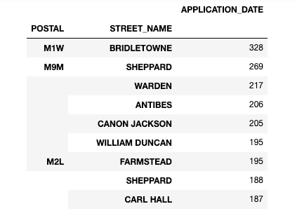
Focusing on new houses and new buildings
let’s take a look at the zip codes and streets with the most permit applications. later on we’ll talk about how this can be important.
new_buildings = permits[permits["PERMIT_TYPE"].isin(["New Building","New Houses"])]
active_zips =  new_buildings.groupby(["POSTAL","STREET_NAME"]).agg({"APPLICATION_DATE":"count"})\
														.sort_values("APPLICATION_DATE",ascending=False)
display(active_zips.iloc[1:100])
zips = permits["POSTAL"].unique()

array(['M2R', 'M4L', 'M6R', 'M6K', 'M6H', 'M5C', 'M4K', 'M6P', 'M2N',
       'M2P', 'M1S', 'M6B', 'M9C', 'M5B', 'M2J', '   ', 'M5J', 'M8V',
       'M5P', 'M3A', 'M5G', 'M5T', 'M4G', 'M3M', 'M9W', 'M8Z', 'M5M',
       'M4M', 'M4E', 'M6J', 'M6G', 'M4Y', 'M5V', 'M2L', 'M8Y', 'M4W',
       'M4N', 'M6L', 'M9A', 'M4V', 'M5N', 'M2M', 'M1L', 'M4T', 'M6S',
       'M6C', 'M5A', 'M4C', 'M9B', 'M3C', 'M5S', 'M4B', 'M9V', 'M1P',
       'M6A', 'M4A', 'M6E', 'M6N', 'M8X', 'M4P', 'M3B', 'M3H', 'M4R',
       'M6M', 'M5H', 'M3J', 'M9M', 'M8W', 'M1C', 'M2H', 'M9R', 'M9N',
       'M4J', 'M1E', 'M5R', 'M4X', 'M3N', 'M4S', 'M5E', 'M5X', 'M2K',
       'M9L', 'M1X', 'M1B', 'M3L', 'M3K', 'M9P', 'M1N', 'M1T', 'M1G',
       'M1K', 'M7A', 'M1J', 'M1H', 'M1R', 'M1M', 'M1W', 'M4H', 'M1V'],
      dtype=object)
Most active zip codes over time
here we start by finding and sorting the most active zip codes, based on the total number of applications. and then we get the top 10 and look into their trend over time. filtering out the most active zip codes gives us meaningful trends.
most_active_zips = new_buildings.groupby(["POSTAL"])\
																.agg({"APPLICATION_DATE":"count"})\
																.sort_values("APPLICATION_DATE",ascending=False)

most_active_zips = most_activezips.index[1:10]
Daily_Count_zipcodes = new_buildings.groupby([pd.Grouper(key="APPLICATION_DATE",freq="M"),"POSTAL"])\
																		.agg({"POSTAL":"count"})

Daily_Count_zipcodes.columns = ["POSTAL_COUNT"]
Daily_Count_zipcodes.reset_index(1,inplace=True)
# Daily_Count_zipcodes
fig, ax = plt.subplots(1,figsize=(20,15))

for zip_code in most_active_zips:
    Daily_Count_zipcodes[Daily_Count_zipcodes["POSTAL"]==zip_code]["POSTAL_COUNT"]\
                                    .rolling(20).mean().plot(ax=ax,label=zip_code)

ax.set_xlim(left=pd.Timestamp("2007-01-01"))
plt.legend( prop={'size': 24})
plt.xticks(fontsize=24)